How to Get Rid of Duplicates in Excel
Learn all of the different ways to remove duplicates in Excel so you can clean up your data and extract useful information.

Excel is excellent software for managing, editing, and manipulating data in various ways. Regardless of your job or field of expertise, you’ll probably have to use Excel at one point or another. That’s why we’re here with our trusty Excel guides to help you nail down the basics. In this guide, we’ll be looking at how to get rid of duplicates in Excel.
It’s common to have columns of data that have duplicate data. Whether it’s people’s names, numbers, locations, or anything in-between, there’s an easy way to check for duplicates in Excel and get rid of them if that’s your goal. That said, removing duplicates is one of the most common uses for Excel, so we’ll show you a few different methods you can add to your Excel toolbelt.
How to Get Rid of Duplicates in Excel
The two ways to get rid of duplicates in Excel are:
- Remove Duplicates button
- Pivot Tables
Remove Duplicates Button
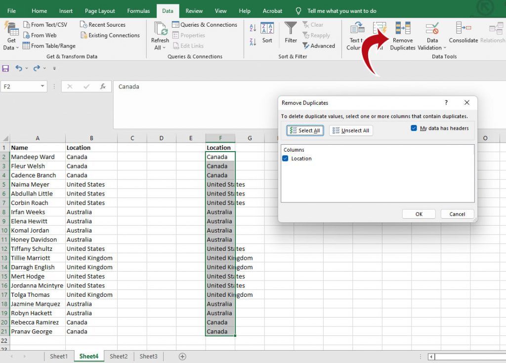
The simplest way to remove duplicates in Excel is by using the Remove Duplicates button. To use Remove Duplicates:
- Highlight the data for which you want to remove the duplicates.
- Navigate to the Data tab in Excel.
- Find and click on the Remove Duplicates button in the Data Tools section.
- Confirm your selection and press OK.
The Remove Duplicates button is the easiest way to remove multiple occurrences of the same word, name, or anything else. To utilize this method efficiently, we recommend preserving your original set of data and copying over the data you want to manipulate.
In the example below, we have two columns: one for name and one for location. We want to remove duplicate locations, so we copy and paste the location data to a new column and click the Remove Duplicates button for that new column.
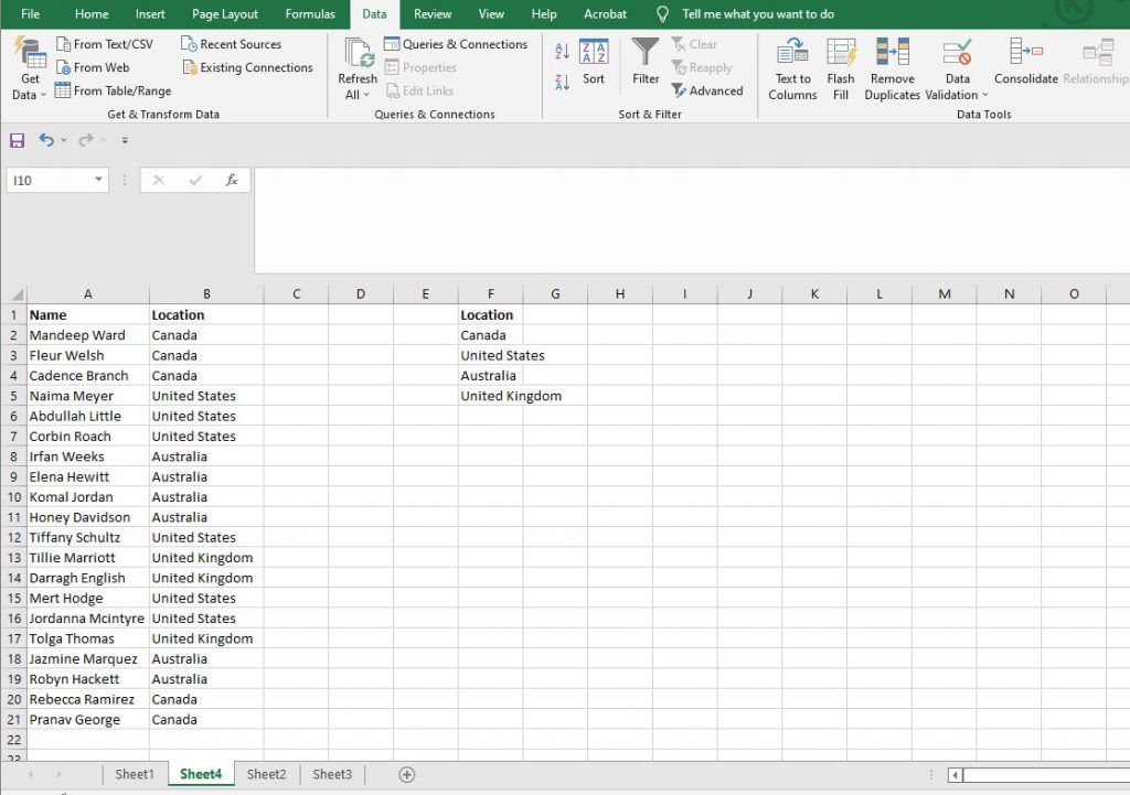
In this example, we were able to get a full list of all the countries without any duplicates. Despite there being 20 rows of data, only four unique countries are mentioned here.
Pivot Tables
Pivot Tables can be used to remove duplicates in Excel. To create a Pivot Table in Excel:
- Highlight the data range for which you want to create a Pivot Table.
- Navigate to the Insert tab in Excel.
- Find and click the PivotTable button.
- Confirm the data range and choose where you want to paste the Pivot Table.
- Press OK to generate the Pivot Table.
- Select the PivotTable Field you want to add to the report.
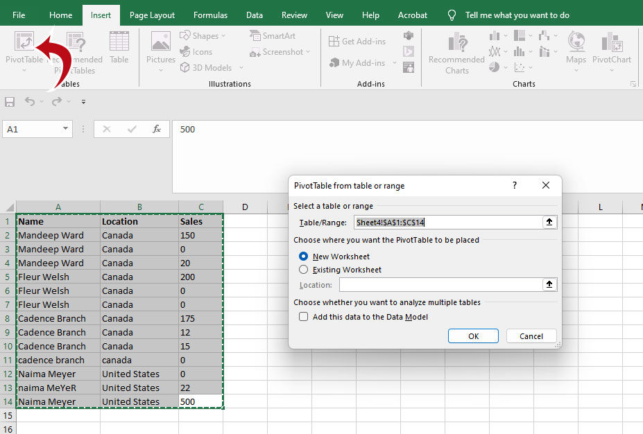
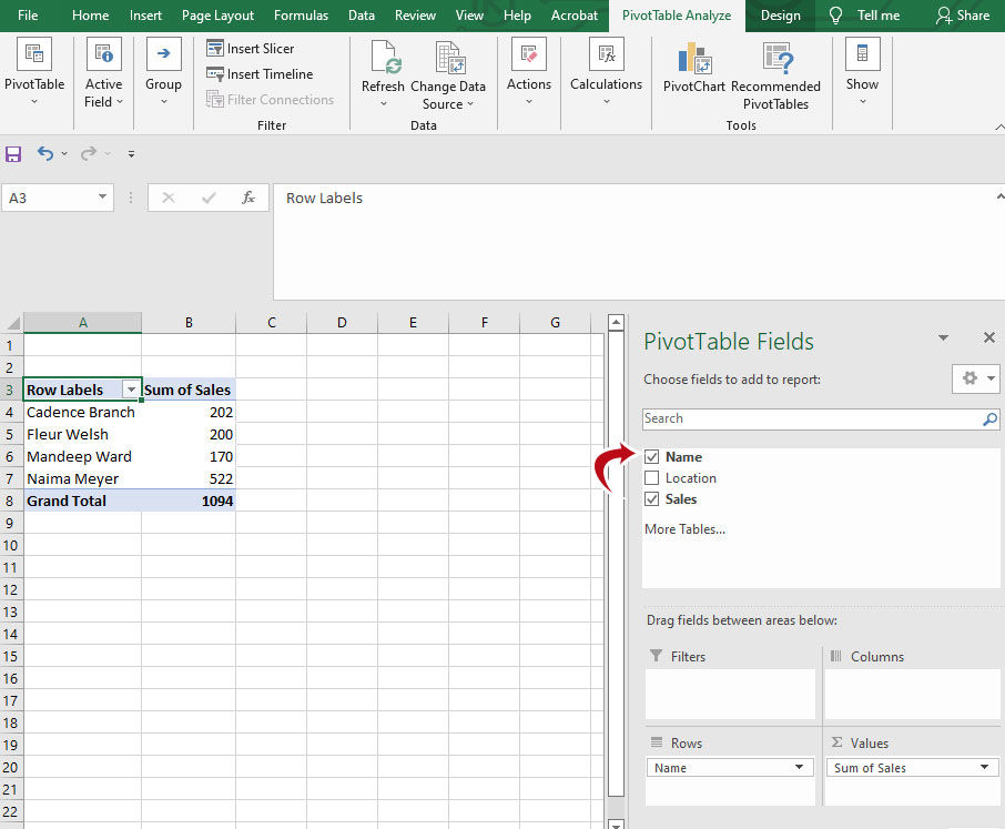
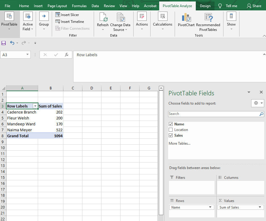
First, make sure your data has headers, as we will use them to organize the data inside the Pivot Table. In the example we’re working with, we have three column headers: Name, Location, and Sales. After highlighting the data and generating a Pivot Table, we can add the fields. If we want to look at name and sales, we will select Name and Sales from the “PivotTable Fields” section.
As a result, we get a list of names without duplicates and a sum of each person’s sales. You can copy and paste the list of names from the Pivot Table if you need to use them for other purposes.
Generally, this is a good solution if you are working with a lot of data. The Pivot Table solution can be valuable if you are looking to remove duplicates and add up data for each occurrence. For example, if a name is mentioned five times and has unique data in each occurrence, you can create a pivot table to add them all up for you.
That’s all you need to know about how to remove duplicates in Excel. You may also want to check out our post on checking for duplicates in Excel.