How to Check for Duplicates in Excel
Learn how to check for duplicates in Excel, so you can better organize your data and get the information you need.

Excel is the leading spreadsheet software next to Google Sheets, and it’s an application used in many fields of work. When working with large sets of data, it is sometimes important to know if the data contains duplicates. But, how do you check for that? This guide will show you easy ways to check for duplicates in Excel to organize your data better.
How to Check for Duplicates in Excel
To check for duplicates in Excel:
- Sort your data.
- Use the COUNTIF function.
Sorting your data
To sort your data in Excel:
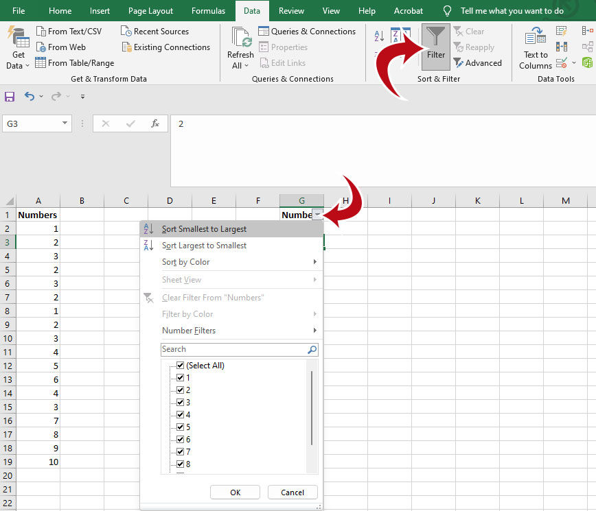
- Highlight the data you want to manipulate.
- Navigate to the Data tab in Excel.
- Click on the Filter button in the Sort & Filter section.
- Tap the dropdown in the header of the data column.
- Sort by smallest or largest (ascending or descending).
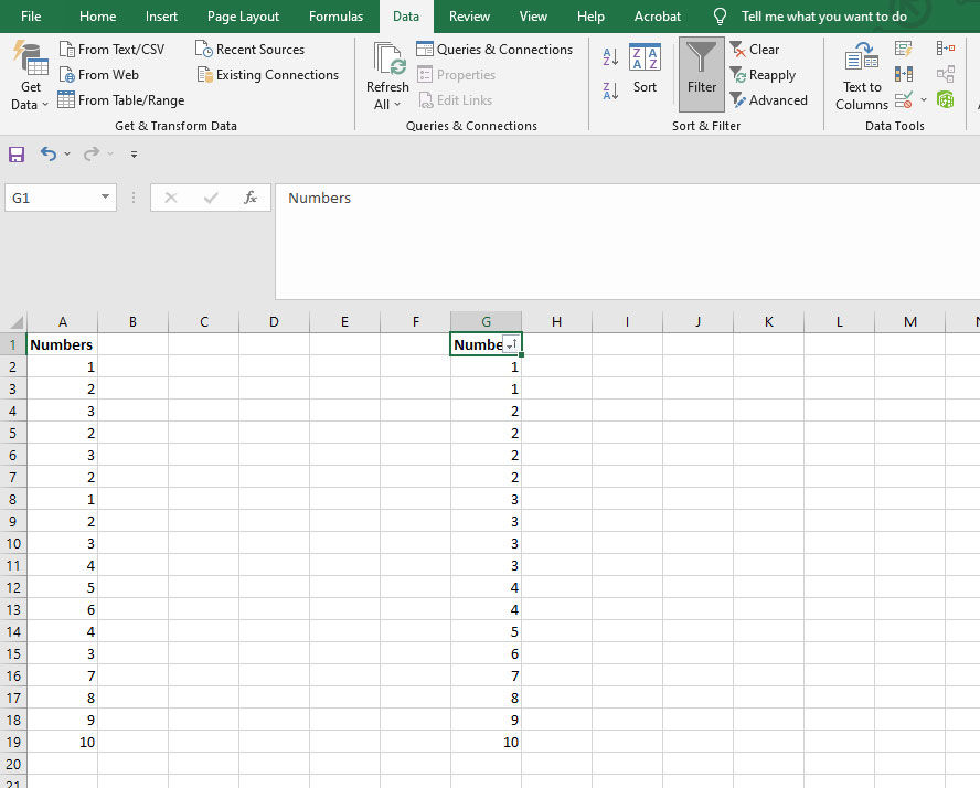
The easiest way to check for data is to sort it in ascending or descending order. Sorting data allows you to visually see if there are duplicates because they will be next to each other in the list. It is a sloppy way to check for duplicates, and it is not viable for larger data sets. Manually identifying duplicates with your eyes can be straining and time-consuming.
That said, sorting your data can be a quick and easy way to check for duplicates if the data you’re working with is small and manageable. For larger data sets, you’re better off trying the other solutions.
Using the COUNTIF function
The best way to check for duplicates in excel is by using the handy COUNTIF function. The function counts cells according to the criteria you enter.
To use the COUNTIF function in Excel to check for duplicates:
- Create another column to the right of your data.
- Enter =COUNTIF and select your range and criteria.
- Autofill the values to check all of the data.
In this example, we use the COUNTIF function to tell us how many times a piece of data appears more than once in a list. We recommend creating a new column to the right of the data you’re manipulating. Label this column “Duplicates” or something to that effect. For simplicity, let’s assume we have one column of data (column B), and our “Duplicate” column is column C.
In cell C2, we will use this equation:
=COUNTIF(B2:B19,B2)
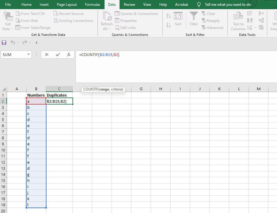
The B2:B19 portion of the function is our data range. The B2 portion of the function is our criteria and references the first piece of data in our list. Press enter to submit the function and double-click the small green box to the bottom right of the cell we just created to autofill the function for the remaining cells.
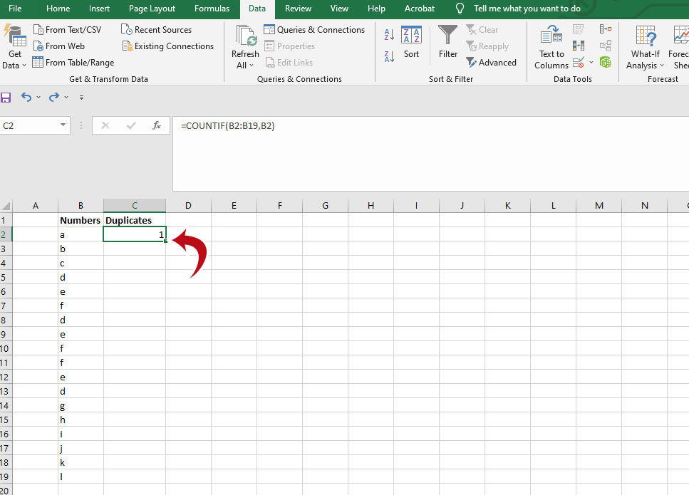
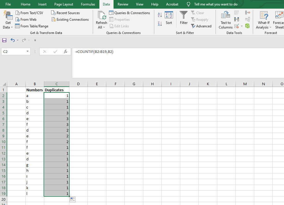
Voila, we now have a column that tells us how many times the value occurs in the list. For example, the letters d, e, and f appear three times each. You can now sort this in descending order to see which values occur most. To take it a step further, you can conditionally format the list to change the color of any value over one.
Adding conditional formatting for duplicate data
To add conditional formatting to highlight duplicate data:
- Go to the Home tab in Excel.
- Tap on Conditional Formatting.
- Choose New Rule.
- Select Use a formula to determine which cells to format.
- Enter $N2>1, where N is your duplicate check column.
- Select a formatting to apply for values greater than one.
- Press OK.
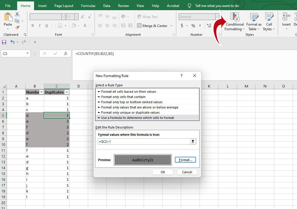
Now all of our duplicate data is highlighted, which makes it easier to identify visually.
Now that you know how to check for duplicates in Excel, you can check out our guide on how to remove duplicates from Excel.