How to Freeze Headers in Google Sheets
Learn how to freeze rows or headers in large Google Sheets documents containing lots of data in just a few simple steps.
Google Sheets is a powerful productivity tool with nearly the same features as Microsoft Excel. When you start working with extensive datasets, you may find the need to make sure that the top header row is frozen in place. Freezing a row allows you to scroll down your document and still see the labels in the first row of each column. This article will look at how to freeze rows in Google Sheets.
As mentioned, freezing the top row can be good practice. If you have a large amount of data that is hundreds of rows long and several columns wide, you may lose your place while scrolling through the data. Locking the topmost data set containing the labels will help you keep track of what you’re doing.
How to Freeze Headers in Google Sheets
To freeze headers in Google Sheets, you need to:
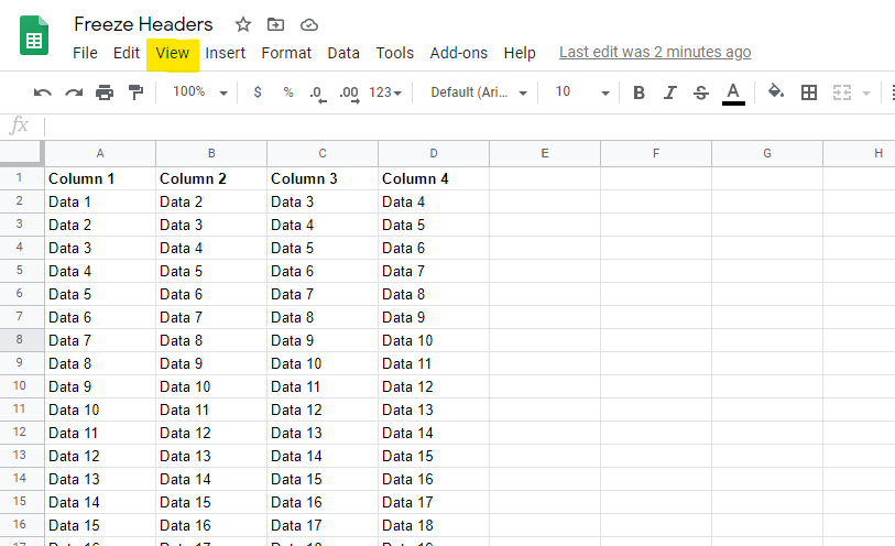
- Click on View
Click on View from the top menu
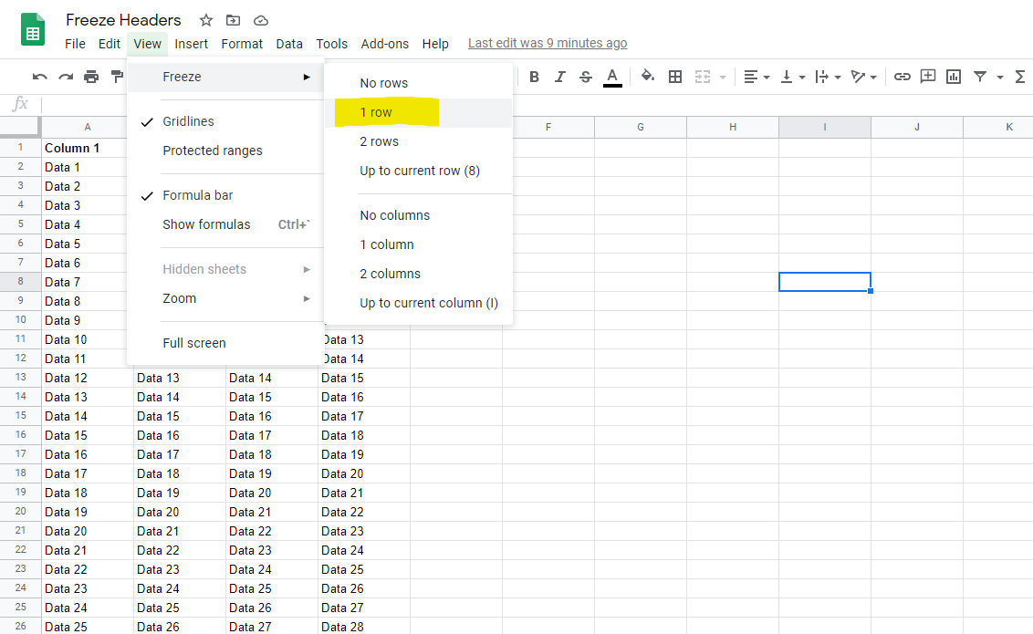
- Click on Freeze
Click on Freeze to open the Freeze options
- Choose Freeze Option
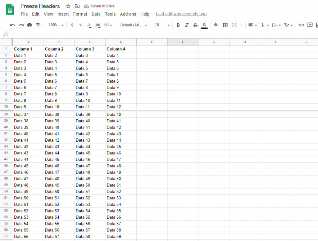
Now choose how many rows you would like to freeze. 1 row is the standard option.
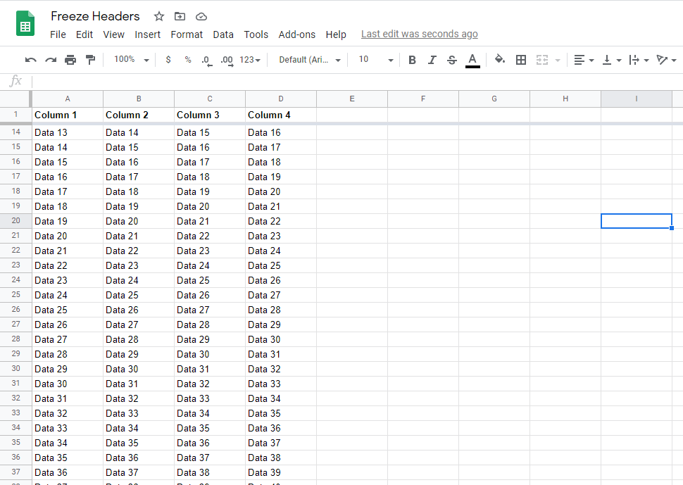
After freezing a row you will see a thicker bottom border on that row, indicating that the row is frozen.
If you would like to freeze two or more rows, you need to:
- Select the row you would like to freeze up to
- Go to View -> Freeze
- Click Up to current row
That’s everything you need to know about how to freeze rows and headers in Google Sheets. Hopefully, this helps you out if you find yourself consistently losing your spot.