How to Compare Two Columns in Excel
Excel can sometimes be tricky. In this article, we review how you can compare two columns in Excel.

If you have a large data set, comparing all of it can become pretty overwhelming. Luckily, Microsoft makes it relatively easy to compare two columns in Excel. This guide will show you a straightforward way to compare data.
How to Compare Two Columns In Excel
What you’ll do depends on the goal of what you’re trying to accomplish with the data. Are you trying to find duplicate entries in each column? Are you looking for mismatched data in the columns? Your goals will affect what steps you choose.
Before we get started, make sure to backup your file before we begin so that way, if you make a mistake, you’ll always have the raw data.
Comparing Two Columns in Excel for Duplicate Entries
We’ll want to use Conditional Formatting and the Highlight tools to determine where our duplicate data is. Follow these steps to highlight duplicate data in two columns.
- Highlight the columns you want to compare.
- In the Home tab, click Conditional Formatting.
- Hover over Highlight Cell Rules.
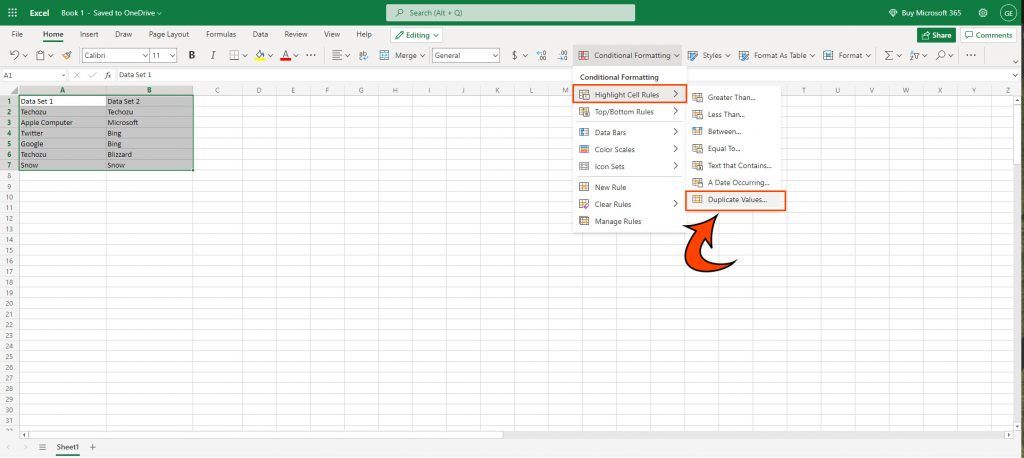
- Click Duplicate Values.
- Select the color you want to use for your highlight.
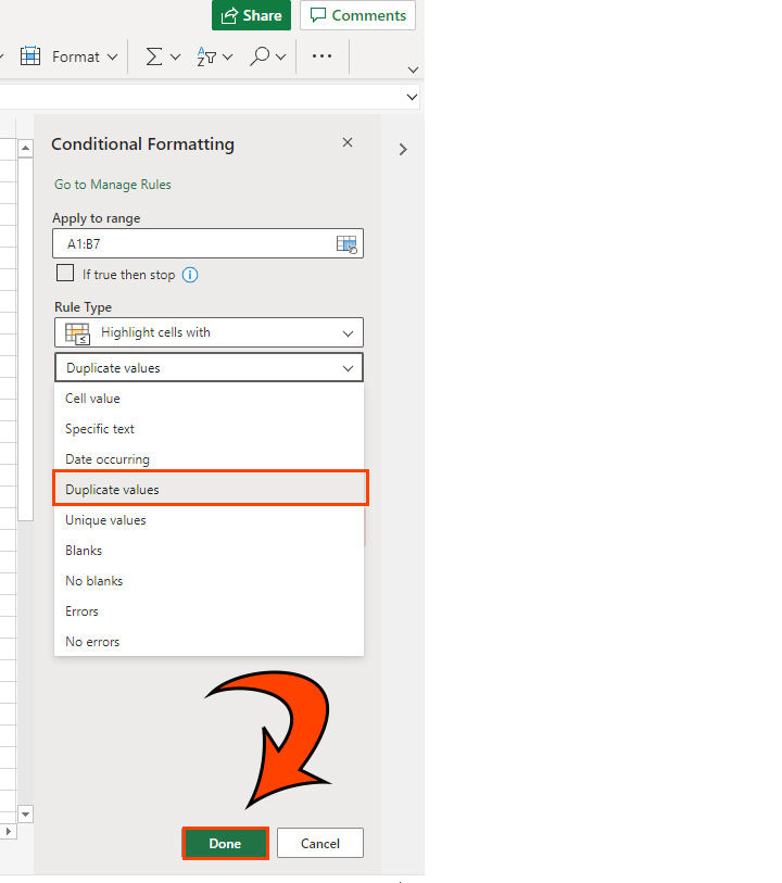
- Click Done.
And that’s it! You’ve now selected all duplicate items in your spreadsheet.
Comparing Two Columns in Excel for Unique Entries
If you instead want to find Unique values, all you have to do is select Unique in the dropdown bar.
- Highlight the columns you want to compare.
- In the Home tab, click Conditional Formatting.
- Hover over Highlight Cell Rules.
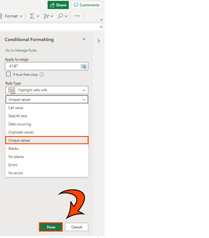
- Click Unique Values.
- Select the color you want to use for your highlight.
- Click Done.
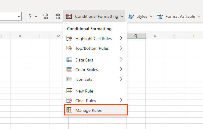
Re-visit your conditional formatting rules later by selecting Conditional Formatting>Manage Rules.
Compare Two Columns in Excel Using an Equals Formula
This technique is a straightforward way to run a quick match on column cells in Excel to get a TRUE or FALSE value on whether your column data matches.
- Click cell C2 or whatever blank cell is adjacent to your last column.
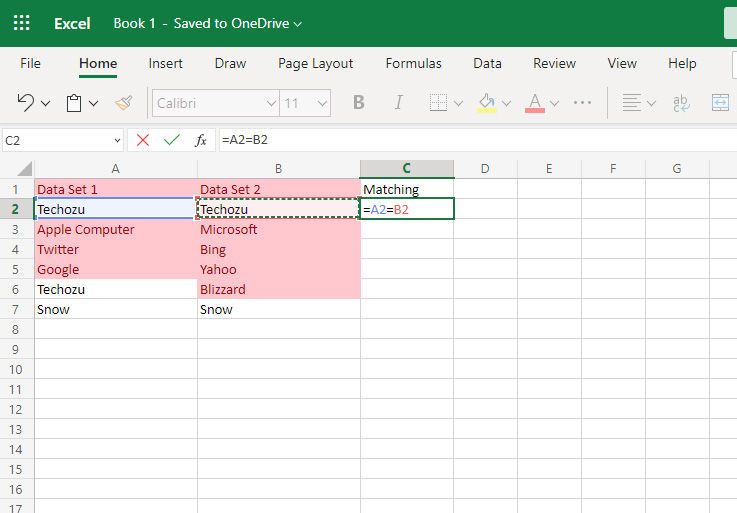
- Type =A2=B2 and hit Enter.
- If you want to compare more than these rows, select the rows you want to compare.
- This gives you a TRUE or FALSE statement on whether your column’s data matches.
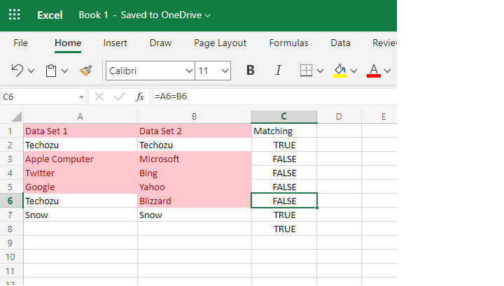
- Copy the formula to the rest of the column by clicking and dragging down on the bottom right of the C2 cell.
You should now have a new column with TRUE and FALSE statements. If TRUE, it means your data matches; if FALSE, it doesn’t.
Hopefully, this helped you compare the data between two different columns in Microsoft Excel.
There are so many use cases for Excel that it can get tricky. If you’re still having issues, head over to our Excel Guides.


